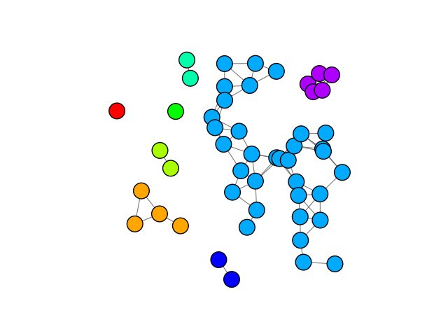
Connected Components

This example demonstrates how to visualise the connected components in a graph using igraph.GraphBase.connected_components().

import igraph as ig
import matplotlib.pyplot as plt
import random

First, we generate a randomized geometric graph with random vertex sizes. The seed is set to the example is reproducible in our manual: you don’t really need it to understand the concepts.

random.seed(0)
g = ig.Graph.GRG(50, 0.15)

Now we can cluster the graph into weakly connected components, i.e. subgraphs that have no edges connecting them to one another:

components = g.connected_components(mode='weak')

Finally, we can visualize the distinct connected components of the graph:

fig, ax = plt.subplots()
ig.plot(
    components,
    target=ax,
    palette=ig.RainbowPalette(),
    vertex_size=0.07,
    vertex_color=list(map(int, ig.rescale(components.membership, (0, 200), clamp=True))),
    edge_width=0.7
)
plt.show()

Note

We use the integers from 0 to 200 instead of 0 to 255 in our vertex colors, since 255 in the igraph.drawing.colors.RainbowPalette corresponds to looping back to red. This gives us nicely distinct hues.