Generating Cluster Graphs

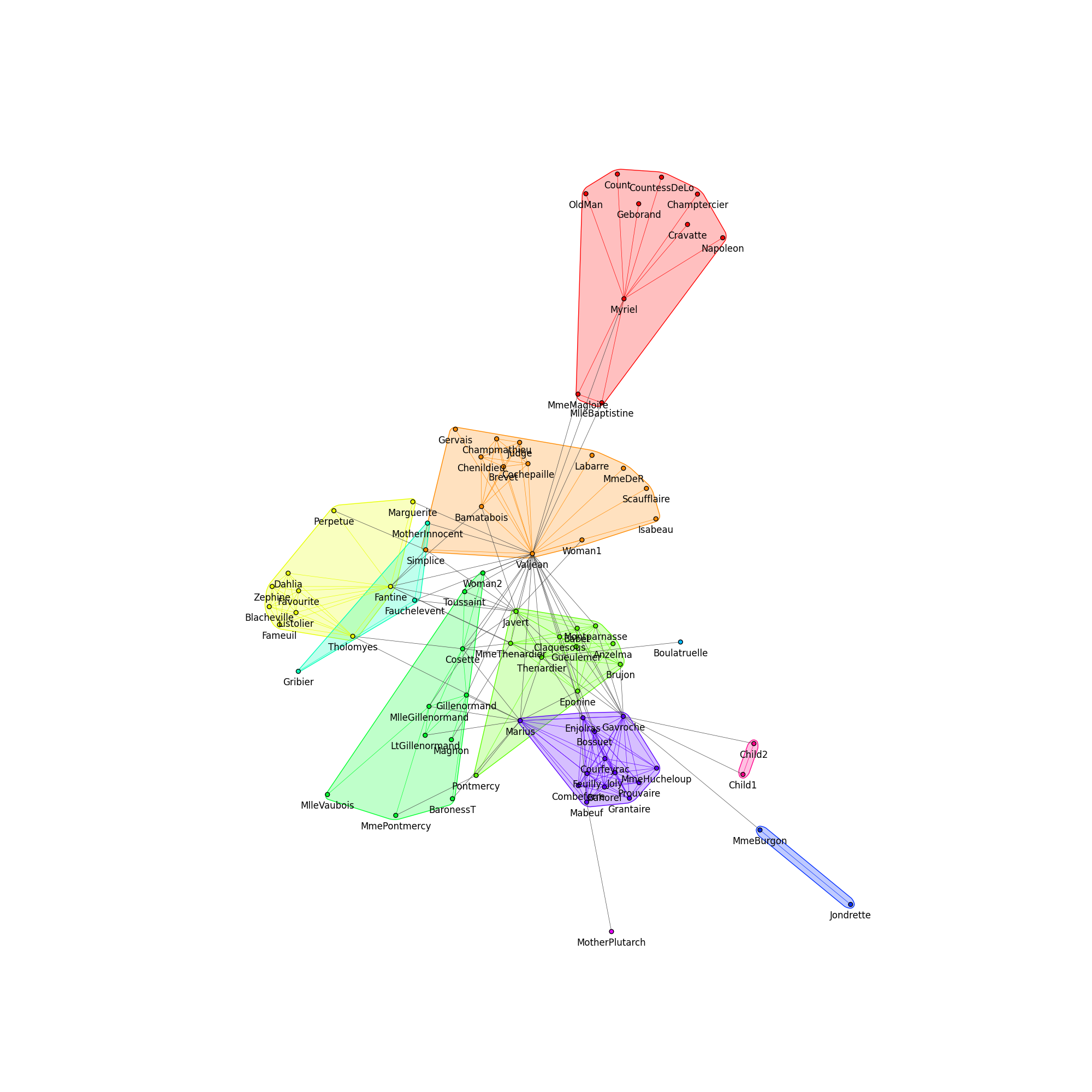
This example shows how to find the communities in a graph, then contract each community into a single node using igraph.clustering.VertexClustering. For this tutorial, we’ll use the Donald Knuth’s Les Miserables Network, which shows the coapperances of characters in the novel Les Miserables.

import igraph as ig
import matplotlib.pyplot as plt

We begin by load the graph from file. The file containing this network can be downloaded here.

g = ig.load("./lesmis/lesmis.gml")

Now that we have a graph in memory, we can generate communities using igraph.Graph.community_edge_betweenness() to separate out vertices into clusters. (For a more focused tutorial on just visualising communities, check out Communities).

communities = g.community_edge_betweenness()

For plots, it is convenient to convert the communities into a VertexClustering:

communities = communities.as_clustering()

We can also easily print out who belongs to each community:

for i, community in enumerate(communities):
    print(f"Community {i}:")
    for v in community:
        print(f"\t{g.vs[v]['label']}")

Community 0:
        Myriel
        Napoleon
        MlleBaptistine
        MmeMagloire
        CountessDeLo
        Geborand
        Champtercier
        Cravatte
        Count
        OldMan
Community 1:
        Labarre
        Valjean
        MmeDeR
        Isabeau
        Gervais
        Bamatabois
        Simplice
        Scaufflaire
        Woman1
        Judge
        Champmathieu
        Brevet
        Chenildieu
        Cochepaille
Community 2:
        Marguerite
        Tholomyes
        Listolier
        Fameuil
        Blacheville
        Favourite
        Dahlia
        Zephine
        Fantine
        Perpetue
Community 3:
        MmeThenardier
        Thenardier
        Javert
        Pontmercy
        Eponine
        Anzelma
        Gueulemer
        Babet
        Claquesous
        Montparnasse
        Brujon
Community 4:
        Cosette
        Woman2
        Gillenormand
        Magnon
        MlleGillenormand
        MmePontmercy
        MlleVaubois
        LtGillenormand
        BaronessT
        Toussaint
Community 5:
        Fauchelevent
        MotherInnocent
        Gribier
Community 6:
        Boulatruelle
Community 7:
        Jondrette
        MmeBurgon
Community 8:
        Gavroche
        Marius
        Mabeuf
        Enjolras
        Combeferre
        Prouvaire
        Feuilly
        Courfeyrac
        Bahorel
        Bossuet
        Joly
        Grantaire
        MmeHucheloup
Community 9:
        MotherPlutarch
Community 10:
        Child1
        Child2

Finally we can proceed to plotting the graph. In order to make each community stand out, we set “community colors” using an igraph palette:

num_communities = len(communities)
palette1 = ig.RainbowPalette(n=num_communities)
for i, community in enumerate(communities):
    g.vs[community]["color"] = i
    community_edges = g.es.select(_within=community)
    community_edges["color"] = i

We can use a dirty hack to move the labels below the vertices ;-)

g.vs["label"] = ["\n\n" + label for label in g.vs["label"]]

Finally, we can plot the communities:

fig1, ax1 = plt.subplots()
ig.plot(
    communities,
    target=ax1,
    mark_groups=True,
    palette=palette1,
    vertex_size=0.1,
    edge_width=0.5,
)
fig1.set_size_inches(20, 20)

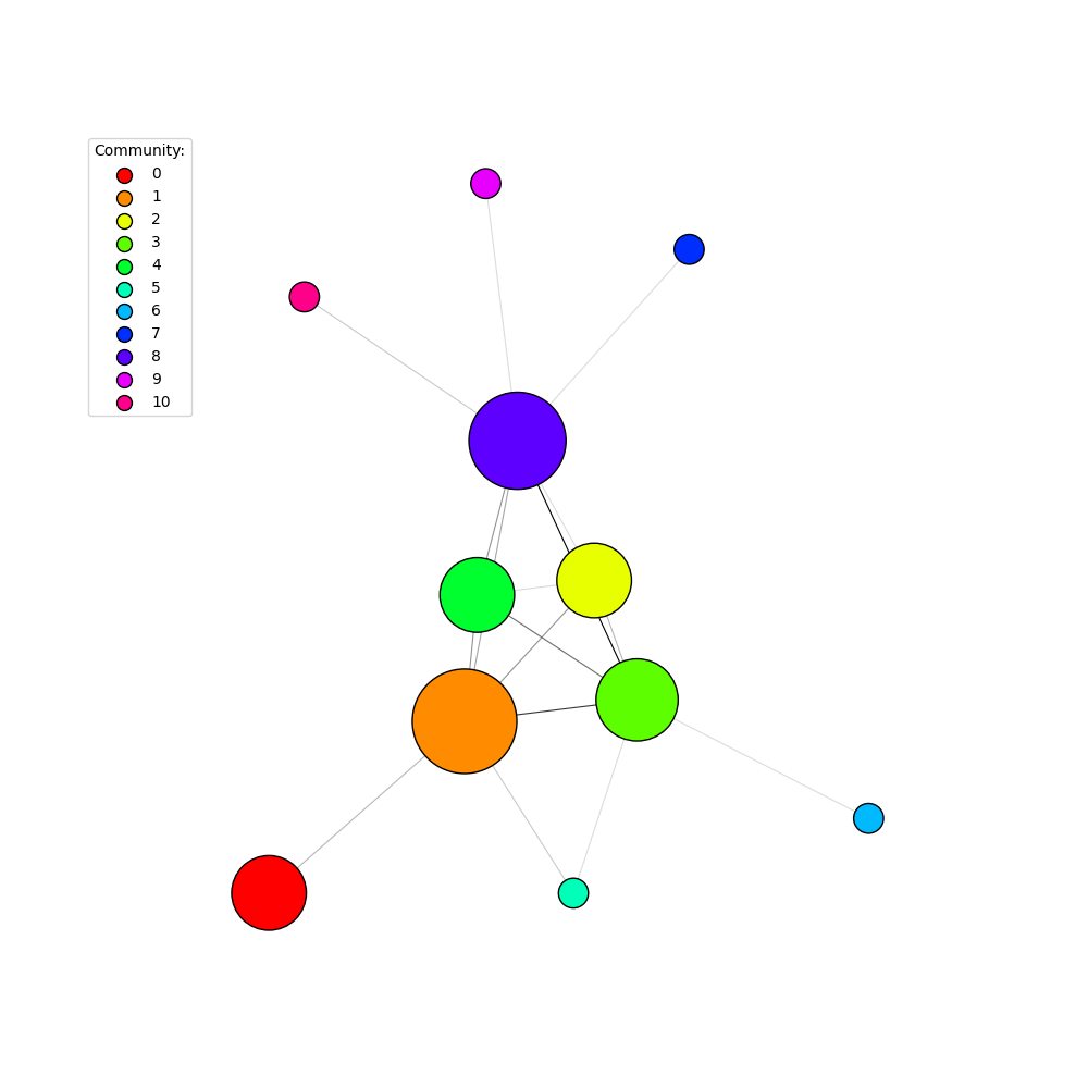
Now let’s try and contract the information down, using only a single vertex to represent each community. We start by defining x, y, and size attributes for each node in the original graph:

layout = g.layout_kamada_kawai()
g.vs["x"], g.vs["y"] = list(zip(*layout))
g.vs["size"] = 1
g.es["size"] = 1

Then we can generate the cluster graph that compresses each community into a single, “composite” vertex using igraph.VertexClustering.cluster_graph():

cluster_graph = communities.cluster_graph(
    combine_vertices={
        "x": "mean",
        "y": "mean",
        "color": "first",
        "size": "sum",
    },
    combine_edges={
        "size": "sum",
    },
)

Note

We took the mean of x and y values so that the nodes in the cluster graph are placed at the centroid of the original cluster.

Note

mean, first, and sum are all built-in collapsing functions, along with prod, median, max, min, last, random. You can also define your own custom collapsing functions, which take in a list and return a single element representing the combined attribute value. For more details on igraph contraction, see igraph.GraphBase.contract_vertices().

Finally, we can assign colors to the clusters and plot the cluster graph, including a legend to make things clear:

palette2 = ig.GradientPalette("gainsboro", "black")
g.es["color"] = [palette2.get(int(i)) for i in ig.rescale(cluster_graph.es["size"], (0, 255), clamp=True)]

fig2, ax2 = plt.subplots()
ig.plot(
    cluster_graph,
    target=ax2,
    palette=palette1,
    # set a minimum size on vertex_size, otherwise vertices are too small
    vertex_size=[max(0.2, size / 20) for size in cluster_graph.vs["size"]],
    edge_color=g.es["color"],
    edge_width=0.8,
)

# Add a legend
legend_handles = []
for i in range(num_communities):
    handle = ax2.scatter(
        [], [],
        s=100,
        facecolor=palette1.get(i),
        edgecolor="k",
        label=i,
    )
    legend_handles.append(handle)

ax2.legend(
    handles=legend_handles,
    title='Community:',
    bbox_to_anchor=(0, 1.0),
    bbox_transform=ax2.transAxes,
)

fig2.set_size_inches(10, 10)