Note
Click here to download the full example code
Complement
This example shows how to generate the complement graph of a graph (sometimes known as the anti-graph) using igraph.GraphBase.complementer().
import igraph as ig
import matplotlib.pyplot as plt
import random
First, we generate a random graph
random.seed(0)
g1 = ig.Graph.Erdos_Renyi(n=10, p=0.5)
Note
We set the random seed to ensure the graph comes out exactly the same each time in the gallery. You don’t need to do that if you’re exploring really random graphs ;-)
Then we generate the complement graph:
g2 = g1.complementer(loops=False)
The union graph of the two is of course the full graph, i.e. a graph with edges connecting all vertices to all other vertices. Because we decided to ignore loops (aka self-edges) in the complementer, the full graph does not include loops either.
g_full = g1 | g2
In case there was any doubt, the complement of the full graph is an empty graph, with the same vertices but no edges:
g_empty = g_full.complementer(loops=False)
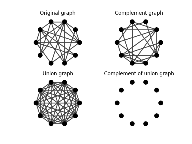
To demonstrate these concepts more clearly, here’s a layout of each of the four graphs we discussed (input, complement, union/full, complement of union/empty):
fig, axs = plt.subplots(2, 2)
ig.plot(
    g1,
    target=axs[0, 0],
    layout="circle",
    vertex_color="black",
)
axs[0, 0].set_title('Original graph')
ig.plot(
    g2,
    target=axs[0, 1],
    layout="circle",
    vertex_color="black",
)
axs[0, 1].set_title('Complement graph')

ig.plot(
    g_full,
    target=axs[1, 0],
    layout="circle",
    vertex_color="black",
)
axs[1, 0].set_title('Union graph')
ig.plot(
    g_empty,
    target=axs[1, 1],
    layout="circle",
    vertex_color="black",
)
axs[1, 1].set_title('Complement of union graph')
plt.show()
Total running time of the script: ( 0 minutes 0.283 seconds)