Betweenness

This example demonstrates how to visualize both vertex and edge betweenness with a custom defined color palette. We use the methods igraph.GraphBase.betweenness() and igraph.GraphBase.edge_betweenness() respectively, and demonstrate the effects on a standard Krackhardt Kite graph, as well as a Watts-Strogatz random graph.

import random
import matplotlib.pyplot as plt
from matplotlib.cm import ScalarMappable
from matplotlib.colors import LinearSegmentedColormap, Normalize
import igraph as ig

We define a function that plots the graph on a Matplotlib axis, along with its vertex and edge betweenness values. The function also generates some color bars on the sides to see how they translate to each other. We use Matplotlib’s Normalize class to ensure that our color bar ranges are correct, as well as igraph’s igraph.utils.rescale() to rescale the betweennesses in the interval [0, 1].

def plot_betweenness(g, vertex_betweenness, edge_betweenness, ax, cax1, cax2):
    '''Plot vertex/edge betweenness, with colorbars

    Args:
        g: the graph to plot.
        ax: the Axes for the graph
        cax1: the Axes for the vertex betweenness colorbar
        cax2: the Axes for the edge betweenness colorbar
    '''

    # Rescale betweenness to be between 0.0 and 1.0
    scaled_vertex_betweenness = ig.rescale(vertex_betweenness, clamp=True)
    scaled_edge_betweenness = ig.rescale(edge_betweenness, clamp=True)
    print(f"vertices: {min(vertex_betweenness)} - {max(vertex_betweenness)}")
    print(f"edges: {min(edge_betweenness)} - {max(edge_betweenness)}")

    # Define mappings betweenness -> color
    cmap1 = LinearSegmentedColormap.from_list("vertex_cmap", ["pink", "indigo"])
    cmap2 = LinearSegmentedColormap.from_list("edge_cmap", ["lightblue", "midnightblue"])

    # Plot graph
    g.vs["color"] = [cmap1(betweenness) for betweenness in scaled_vertex_betweenness]
    g.vs["size"]  = ig.rescale(vertex_betweenness, (0.1, 0.5))
    g.es["color"] = [cmap2(betweenness) for betweenness in scaled_edge_betweenness]
    g.es["width"] = ig.rescale(edge_betweenness, (0.5, 1.0))
    ig.plot(
        g,
        target=ax,
        layout="fruchterman_reingold",
        vertex_frame_width=0.2,
    )

    # Color bars
    norm1 = ScalarMappable(norm=Normalize(0, max(vertex_betweenness)), cmap=cmap1)
    norm2 = ScalarMappable(norm=Normalize(0, max(edge_betweenness)), cmap=cmap2)
    plt.colorbar(norm1, cax=cax1, orientation="horizontal", label='Vertex Betweenness')
    plt.colorbar(norm2, cax=cax2, orientation="horizontal", label='Edge Betweenness')

First, generate a graph, e.g. the Krackhardt Kite Graph:

random.seed(0)
g1 = ig.Graph.Famous("Krackhardt_Kite")

Then we can compute vertex and edge betweenness:

vertex_betweenness1 = g1.betweenness()
edge_betweenness1 = g1.edge_betweenness()

g2 = ig.Graph.Watts_Strogatz(dim=1, size=150, nei=2, p=0.1)
vertex_betweenness2 = g2.betweenness()
edge_betweenness2 = g2.edge_betweenness()

Finally, we plot the two graphs, each with two colorbars for vertex/edge betweenness

fig, axs = plt.subplots(
    3, 2,
    figsize=(7, 6),
    gridspec_kw=dict(height_ratios=(20, 1, 1)),
)
plot_betweenness(g1, vertex_betweenness1, edge_betweenness1, *axs[:, 0])
plot_betweenness(g2, vertex_betweenness2, edge_betweenness2, *axs[:, 1])
fig.tight_layout(h_pad=1)
plt.show()

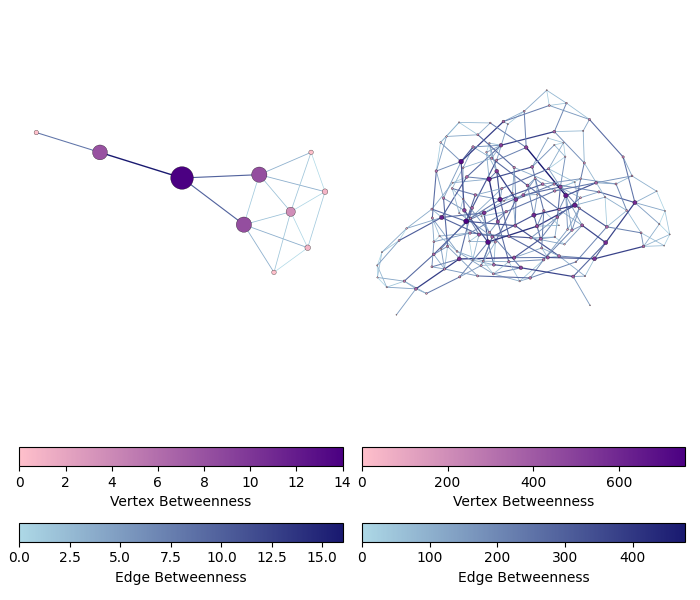
vertices: 0.0 - 14.0
edges: 1.5 - 16.0
vertices: 0.0 - 753.8235063912693
edges: 8.951984126984126 - 477.30745059034535