Visual styling

This example shows how to change the visual style of network plots.

import igraph as ig
import matplotlib.pyplot as plt
import random

To configure the visual style of a plot, we can create a dictionary with the various setting we want to customize:

visual_style = {
    "edge_width": 0.3,
    "vertex_size": 15,
    "palette": "heat",
    "layout": "fruchterman_reingold"
}

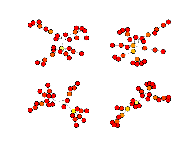
Let’s see it in action! First, we generate four random graphs:

random.seed(1)
gs = [ig.Graph.Barabasi(n=30, m=1) for i in range(4)]

Then, we calculate a color colors between 0-255 for all nodes, e.g. using betweenness just as an example:

betweenness = [g.betweenness() for g in gs]
colors = [[int(i * 255 / max(btw)) for i in btw] for btw in betweenness]

Finally, we can plot the graphs using the same visual style for all graphs:

fig, axs = plt.subplots(2, 2)
axs = axs.ravel()
for g, color, ax in zip(gs, colors, axs):
    ig.plot(g, target=ax, vertex_color=color, **visual_style)
plt.show()

Note

If you would like to set global defaults, for example, always using the Matplotlib plotting backend, or using a particular color palette by default, you can use igraph’s configuration instance :class:`igraph.configuration.Configuration. A quick example on how to use it can be found here: Configuration Instance.

In the matplotlib backend, igraph creates a special container igraph.drawing.matplotlib.graph.GraphArtist which is a matplotlib Artist and the first child of the target Axes. That object can be used to customize the plot appearance after the initial drawing, e.g.:

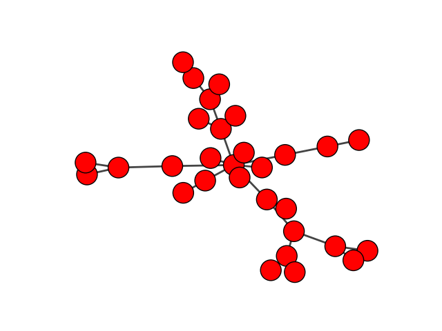
g = ig.Graph.Barabasi(n=30, m=1)
fig, ax = plt.subplots()
ig.plot(g, target=ax)
artist = ax.get_children()[0]
# Option 1:
artist.set(vertex_color="blue")
# Option 2:
artist.set_vertex_color("blue")
plt.show()

Note

The igraph.drawing.matplotlib.graph.GraphArtist.set() method can be used to change multiple properties at once and is generally more efficient than multiple calls to specific artist.set_... methods.

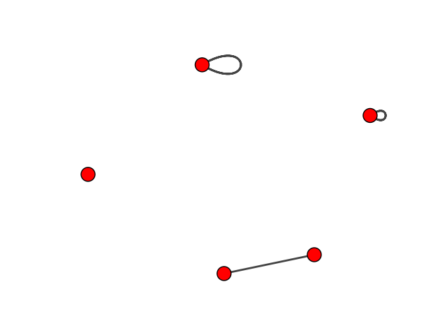
In the matplotlib backend, you can also specify the size of self-loops, either as a number or a sequence of numbers, e.g.:

g = ig.Graph(n=5)
g.add_edge(2, 3)
g.add_edge(0, 0)
g.add_edge(1, 1)
fig, ax = plt.subplots()
ig.plot(
    g,
    target=ax,
    vertex_size=20,
    edge_loop_size=[
        0,  # ignored, the first edge is not a loop
        30,  # loop for vertex 0
        80,  # loop for vertex 1
    ],
)
plt.show()